We have covered enough probability theory at this point to begin our discussion of statistics. Probability and statistics are complementary approaches to the same problem of describing phenomena which are recalcitrant to deterministic treatment. Probability theory asks "given a model (probabilistic) of this phenomena, what can be said about the data that I might expect from experiments (or observations) performed on this system"? Statistics, on the other hand, asks "given data generated from experiments (or observations) on this system, what can I say about a model for this phenomenon"? Hopefully, you appreciate the close kinship of these two fields of study and are consequently full of forgiveness for the preceding 12 pages of introductory probability theory.
Statistics is a big field, and therefore we will be able to address only one small topic within the space of these notes. This is meant both as an apology and encouragement, since there is much more to statistics and you should be familiar with much of it for future work in biology. Apologies aside, the topic that will occupy our attention here is that of hypothesis testing. The name is rather self-explanatory, but the core idea is that we formulate some hypothesis about a population, take a sample of this population, and use the resulting characteristics of this sample to determine the probability that our hypothesis is correct. The hypothesis that we are testing is called the null hypothesis. To test this hypothesis, we take a sample of the population and decide on a test statistic. The test statistic quantifies the agreement between the hypothetical characteristic of the population and the observed characteristic of the sample. Lastly, you compute the probability that your test statistic would have at least the observed value if your hypothesis (the null hypothesis) is correct. The probability is often called a p-value, and if it is below a pre-determined cutoff (usually either 0.05 or 0.01), you decide to reject the null hypothesis. In rejecting the null hypothesis, you are saying that the difference between the hypothesized characteristic of the population and your sample characteristic is too large to be due to "random" fluctuation, and therefore something else that is not accounted for by your null hypothesis must be at work.
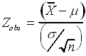
To make all this a bit more concrete, lets consider an example. Suppose you are interested in determining whether a biotech. company is being honest about the activity of an enzyme they are selling. You purchase some enzyme, remove n aliquots and assay each aliquot for activity. The company claims that their enzyme activity is m units/ml. Therefore, your null hypothesis is that the enzyme's mean activity is m units/ml, and is normally distributed about this mean. Therefore, your test statistic in this case is
Where ![]() is the sample mean, and s
is the sample standard deviation.
is the sample mean, and s
is the sample standard deviation.
Essentially, we can view the test statistic as a r.v. which we assume is normally distributed. Therefore, given a computed test statistic, we can use the normal distribution to calculate the probability that the null hypothesis is true. We will do this by computing the probability that the test statistic assumes a value at least as large as that observed. In other words,
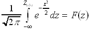
If the p-value is less than a given cutoff (0.05 or 0.01), we conclude that it is improbable that the test statistic would assume such a large value and therefore reject the null hypothesis. In the case of our example, we may find a p-value<0.01, and therefore reject the companys claim concerning the activity of their enzyme. We should note in passing that the details of computing the p-value can vary. There exist two distinct methods of computation; the one-tailed or two-tailed tests. They differ only insofar as the latter test explicitly capitalizes on the symmetry of the standard normal distribution, and consequently, the details of the implementation are slightly different. You need not be overly concerned about this.
In closing our discussion of hypothesis testing, you should note that a test statistic can be constructed to test a wide variety of hypotheses. For example, we could construct a test statistic to determine whether the observed proportion of defective products in a sample is significantly different that the quoted defective rate. Many other such applications exist, and consequently hypothesis testing is among the most commonly employed of statistical methods.
With all this talk about probability and statistics, you may be fearing that deterministic mathematics is totally irrelevant to bioinformatics. This is most certainly not the case. In fact, a mathematical object of great utility in this field is the vector. This is because vectors provide a uniquely powerful way to represent and manipulate large quantities of information. For example, the structure of a biomacromolecule may be thought of as a 3N-dimensional vector, where N is the number of atoms in the structure. In what follows, we will review some of the most important aspects of vector algebra.
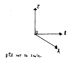
As you recall from physics, vectors are objects that have both magnitude and direction, and are many times represented by arrows to indicate this fact. In doing so, we should see that we can also represent this vector by its components along the x,y and z axes Therefore, in general we have
Where ![]() represents the length (also called magnitude or norm) of our vector,
represents the length (also called magnitude or norm) of our vector, ![]() are the unit vectors (vectors of length=1) that point in along the x, y
and z axes respectively, and
are the unit vectors (vectors of length=1) that point in along the x, y
and z axes respectively, and ![]() are the angles between the vector and the x, y, and z axes, respectively
(as below).
are the angles between the vector and the x, y, and z axes, respectively
(as below).
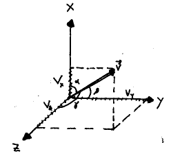
The above illustration shows us that the x,y, and z components of the vector are equivalent to the projection of this vector onto these axes. Since these projections are just the magnitude of the vector multiplied by the cosine of the angle between the vector and the axes, we realize that if we know the length of the vector and the angle it makes to each axis, then we know in what direction to draw the vector. Because these angles tell us in what direction to draw the vector, the cosines of these angles are called the direction cosines. They arise frequently and you should keep in mind that the direction cosines are just another way of representing the components of the vector under consideration. Before we leave the topic of direction cosines, consider the expression for the magnitude of a vector, shown below
This implies
which you should verify.
Just as we can (uniquely) specify a vector by listing its components, we can also operate on vectors via operating on their components. For example, you learned in physics that vectors can be added geometrically using the "head-to-tail" rule for vector addition. Now, if what we just said about operating on vector component-wise is true, it should provide us with the same answer for addition of vectors as does "head-to-tail" addition. We verify this geometrically below
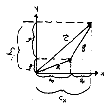
Therefore ![]() .
We can see that as the number of vectors increases, it becomes much more
difficult to draw them all out and do "head-to-tail" addition. In contrast,
adding 10 numbers is not much harder than is adding 2. Therefore, the great
advantage of component-wise addition of vectors is that it allows us to
reduce the potentially tedious problem of adding arrows to the much easier
one of adding numbers.
.
We can see that as the number of vectors increases, it becomes much more
difficult to draw them all out and do "head-to-tail" addition. In contrast,
adding 10 numbers is not much harder than is adding 2. Therefore, the great
advantage of component-wise addition of vectors is that it allows us to
reduce the potentially tedious problem of adding arrows to the much easier
one of adding numbers.
Having conquered vector addition, you may be tempted to apply similar methodology to vector multiplication. Unfortunately, multiplying vectors is trickier than adding them, since there are two ways of forming vector products. One way is very similar to our component-wise method of vector addition, and it produces a number (scalar). Therefore, this method of vector multiplication is called the scalar (or dot) product. The other way of multiplying vectors is very different from straightforward component-wise operation and produces another vector. Consequently, it is called the vector (or cross) product. In what follows, we will take some time to discuss each kind of vector product and its significance.
The dot product of two vectors is given by the following relation
Where q is the angle between these two vectors. The first equality above is useful primarily when actually computing a dot product. The second equality is useful when manipulating vector relations (although it is of considerable computational utility as well). The cosine term in the above suggests a geometric interpretation of the dot product very similar to that given for the direction cosines. Namely, this equality tells us that the dot product of two vectors is the product of the vector magnitudes projected along the direction of one of the vectors. Furthermore, the cosine term allows us to conclude that parallel vectors produce maximal dot products and perpendicular vectors produce zero dot products. Perpendicular vectors are called orthogonal, and are of very general importance. You will see them again in linear algebra, but with a somewhat less geometric interpretation. As a closing comment on the many-faceted wonder of the dot product, you should note that, by virtue of the first equality, the dot product is commutative (order of multiplication does not matter). This is a direct consequence of the commutativity of scalar multiplication.
In contrast to the appealing simplicity of component-wise multiplication that characterizes the dot product, the cross product is a less straightforward matter. We define the cross product as
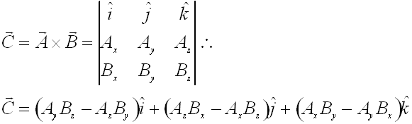
where the bars on either side of the matrix indicate that we are to find the determinant of the matrix inside. Although we are dealing with a topic that more properly belongs in a discussion of linear algebra, lets discuss how to compute the determinant of a matrix.
For most "by hand" computations, a determinant is most easily found by using the so-called "expansion by minors" approach. This is done as shown below
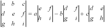
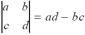
This should seem less than helpful, since we have just broken down one determinant into three. However, finding the determinant of a 2x2 matrix is rather easy. We just multiply the entries lying on "left-to-right" diagonal and subtract the product of the entries lying on the "right-to-left" diagonal. In other words,
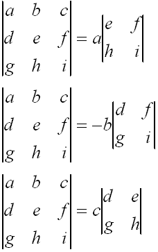
Knowing this, we can introduce a convenient mnemonic device for the computing the determinant of a 3x3 matrix, which we can represent as below
Knowing this, you should expand the determinant of the matrix in (21) and verify that you do indeed get the vector indicated in the second equality in (21).
Now that youre comfortable with how to compute the cross product, a few geometrical considerations are in order. First, the cross product always produces a vector which is perpendicular (orthogonal) to both of the vectors "crossed" in the cross product, as shown below.
In addition, the definition of the cross product in (21) leads us to conclude that the cross product, unlike the dot product, in not commutative. In fact, if we reverse the order of the vectors in (21) and compute the result, we get a vector which points in the opposite direction as the original product. More succinctly,
This property is called anticommutativity. The direction of the resulting vector can be easily remembered using the right-hand rule. The rule says that the product vector will point in the same direction as the thumb on your right hand if you align your palm with the first vector and curl your fingers toward the second vector in the cross product. You probably were introduced to this in physics. In concluding our discussion of the cross product, you should be aware of the following relation between the magnitude of the product vector and the magnitudes of the vectors being crossed. Namely,
You will not make as much use of this as you will (20), but (26) is still worth remembering.
Furthermore, just as we can multiply more than two
scalars, we can also multiply more than two vectors. However, always keep
in mind that the two ways of multiplying vectors (dot and cross product)
that we have just discussed are only defined for vectors. So, while we
can make the triple product ![]() ,
we can not make the triple product
,
we can not make the triple product ![]() ,
since the term in parenthesis is a scalar, and the cross product is only
defined between two vectors. Because this requirement removes the potential
ambiguity in the triple product, parenthesis are usually omitted. The triple
product you are most likely to encounter in future studies is the scalar
triple product, given by
,
since the term in parenthesis is a scalar, and the cross product is only
defined between two vectors. Because this requirement removes the potential
ambiguity in the triple product, parenthesis are usually omitted. The triple
product you are most likely to encounter in future studies is the scalar
triple product, given by
The choice of ![]() to represent this scalar triple product is suggestive. In fact, the scalar
triple product is often used to calculate volumes of parallelepipeds. A
biophysically relevant example would be the volume of the unit cell of
a crystal, which is a very important parameter in crystallography. However,
this is only one of many applications of vectors to biophysics, so please
make sure that you are comfortable with them before you continue.
to represent this scalar triple product is suggestive. In fact, the scalar
triple product is often used to calculate volumes of parallelepipeds. A
biophysically relevant example would be the volume of the unit cell of
a crystal, which is a very important parameter in crystallography. However,
this is only one of many applications of vectors to biophysics, so please
make sure that you are comfortable with them before you continue.
Having treated vectors via their components, it will
come as no surprise to you that we can further "economize" our treatment
of vectors by representing them as lists of components. For example, we
could represent the vector ![]() in any of the three ways shown below.
in any of the three ways shown below.
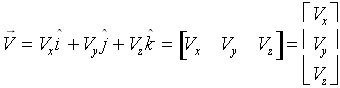
The last two quantities are examples of a row vector and a column vector, respectively. This may seem like dry exposition on bookkeeping methods for vectors, but it allows us to achieve a great simplification in how we handle vectors, to which we turn our attention now.
Consider the vector shown below, which is represented in two coordinate systems, one rotated with respect to the other by f . The problem is to provide expressions for the components of the vector in the new (rotated) coordinate system in terms of its old components.
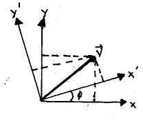
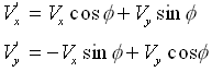
You will need to use the sum formulas from trigonometry to do this problem (and might try it as an exercise). In doing so, you will find the following;
As you have already come to appreciate, this problem is somewhat tedious if solved in the manner suggested above. The great attraction of representing vectors as row or column vectors is that we can operate on these vectors using matrices. However, to do so, we will first need to discuss the anatomy and mechanics of matrices and their manipulation.
A matrix is simply an array of numbers, which are called entries. The entries are organized amongst rows and columns. As you have probably already anticipated, columns run up-down and rows run side-to-side. Therefore, we can uniquely specify an entry in the matrix by providing its row and column index. A generic matrix is shown below
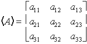
The above matrix is an example of a 3x3 matrix, where, by convention, the first number refers to the number of rows and the second to the number of columns. Matrices may come in any size, 1x3 ( 3-dimensional row vector), 3x1 (3-dimensional column vector), 3x3, 4x2, 100x1734, etc.
We can add matrices entry by entry, as below;
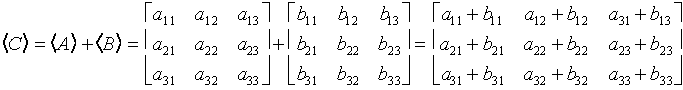
Note that this is exactly analogous to component-wise addition of vectors.
Continuing this analogy with vector algebra, while we can add (and subtract) matrices easily, multiplication is somewhat trickier. In brief, matrix multiplication obeys the following rule
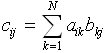 . The product
matrix
. The product
matrix All that this definition is saying is that the element ![]() is
just the
is
just the ![]() row of
row of ![]() multiplied by the
multiplied by the ![]() column
of
column
of ![]() in a component-wise
fashion and then summed. You might recognize that this is similar to the
method of computing the dot product of two vectors. As it turns out, there
is an excellent reason for this similarity because this row-by-column method
of matrix multiplication is perfectly equivalent to the dot product. To
verify this, choose two vectors and compute their dot product. Next, arrange
the components of first vector as a row vector, and the second as a column
vector. Now, perform matrix multiplication as defined above and verify
that the results are identical. In linear algebra, this is called the inner
product.
in a component-wise
fashion and then summed. You might recognize that this is similar to the
method of computing the dot product of two vectors. As it turns out, there
is an excellent reason for this similarity because this row-by-column method
of matrix multiplication is perfectly equivalent to the dot product. To
verify this, choose two vectors and compute their dot product. Next, arrange
the components of first vector as a row vector, and the second as a column
vector. Now, perform matrix multiplication as defined above and verify
that the results are identical. In linear algebra, this is called the inner
product.
Having defined matrix multiplication, we can now re-inspect (29) and recognize that this is equivalent to the matrix equation
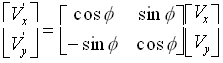
The type of matrix shown in (32) is among the most useful matrices you will ever encounter. It is called a rotation matrix, and given the example that produced it, you should immediately appreciate why. These matrices are used in every imaginable application, and being comfortable with them is critically important.
Now that youve seen a rotation matrix in two dimensions, we will generalize this result to three dimensions. The key to doing this is to imagine rotating a Cartesian (3-D) coordinate system about one of its three orthogonal axes, as below.
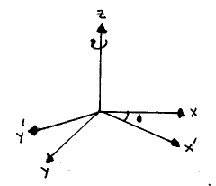
This is equivalent to rotating the xy plane through an angle f while leaving z unchanged. The three dimensional rotation matrix for this operation is
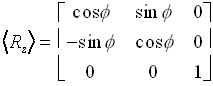
Note that, in matrices of this sort (in a Cartesian basis, to be precise), the first column represents the x-axis, the second the y and the third the z-axis. Here, we are assuming that we are working in a column space.
Now, we could describe an arbitrary three dimensional rotation matrix by considering the consecutive rotations of the coordinate system around z, x, and the "new" z-axis (new in that its orientation has changed with respect to its original position). Such matrices are necessary to describe the orientations of rigid bodies in space relative to some external coordinate system. Therefore, in matrix notation,
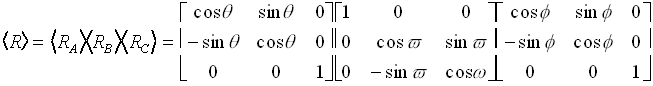
The angles through which we are rotating the coordinates are called the Euler angles. However, two points about the above should be hastily made. First, since matrix multiplication is not commutative (order matters), the order that you perform these rotations is very important. Nearly every field that uses Euler angles has a different convention for order of rotations, so we will not waste space here discussing them all. In addition, this topic is among the most non-intuitive you are likely to encounter with any regularity. Therefore, if youre interested, you should curl up with some classical mechanics textbook and devote a hour or so to serious study. Lastly, we should note that we have just scratched the surface of the elegant field of linear algebra, which finds no end of application in every field of science. It is mandatory that you master elementary linear algebra in order to fully enjoy the mass of biophysically and bioinformatically relevant mathematics.