
Biological systems are, as a rule, large and complicated. This makes it unlikely that deterministic equations which describe these systems in detail will prove useful, because the complexity of these systems will be reflected in a similar complexity in the equations that describe them. Furthermore, since obtaining experimental measurements of the values of the many variables that would appear in such equations is difficult or impossible, we need to simplify our description somewhat if we intend to apply quantitative methods to biological systems. One way that we can accomplish this is by moving from an explicit to an implicit treatment of a great many of the variables that complicate these expressions. In doing so, we choose to model the collective influence of these "ignored variables" on the system by resorting to a probabilistic treatment of these systems. This turns out to be an important and useful simplification, and therefore a brief discussion of probability theory may prove useful to your future work in biology. In addition, it will provide a nice starting point for our later discussion of statistics.
We are used to thinking about probabilities as being a generalization of the notion of the frequency of occurrence of an event, where the probability that the event under consideration occurs is defined as the ratio of the number of favorable outcomes of an experiment to the total number of trials in the limit of an infinite number of trials.

It turns out that this definition is unacceptable from a mathematical point of view, but it provides a fine guide to your intuition, and therefore you should not abandon it entirely. Additionally, if this definition is modified slightly, it proves to be very useful in the computation of probabilities of certain types of events (when there are only a finite number of equiprobable outcomes in the experiment), as we will discuss shortly.
Rather than the above definition, which is mathematically unacceptable because it relies explicitly on empirical observation, we will begin our discussion of probabilities using some notions from set theory. Though it sounds intimidating, set theory is nothing but a more formal version of logic, and you have already used notions from it innumerable times. Just to complicate things somewhat in the beginning, a set, technically speaking, can not be defined because any definition of a set must make use of the notion of a set and is therefore circular. However, technicalities aside, you can think of a set as a collection of objects, which are called elements. As an example, the set of all people in Prof. Gersteins Bioinformatics class is equivalent to the set composed of a list of your names. In addition to being an example of a set, the above also provides a nice illustration of an important notion from set theory, which says that a set may be specified by either providing a condition that all elements of the set satisfy or by enumerating every element of the set. For example, the set of all integers greater than 2 and less than 10 may be written as follows
where the bar should be read "such that" and the "fork" indicates that the quantity to the left are the elements of the set to the right. In addition, the set N is the set of all natural numbers (positive integers). Therefore, the above may be translated "the set S is equal to the elements x such that every element is greater than two and less than 10 and every element is an integer". A bit formal, but necessarily so-set theory is the distillation of logic and is therefore quite formal. In addition, there are two sets that are so important that they deserve special mention. They are the universal set W, which is the set that contains every element under consideration and the null set Æ, which contains no elements (and consequently is sometimes called the empty set).
Having defined sets, we can perform some basic operations with them. Given two sets A and B, we define three operations called intersection, union and complement. Introducing some more notation,
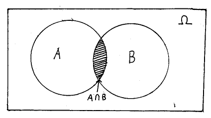
A few words are in order about the above. The intersection of two sets produces a third set whose elements are only those elements that are common to both sets A and B. This is most easily understood using a Venn diagram, as shown below
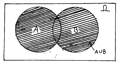
Next, the union of two sets produces a third set whose elements are those that were contained in either set A or set B, or both, as below.
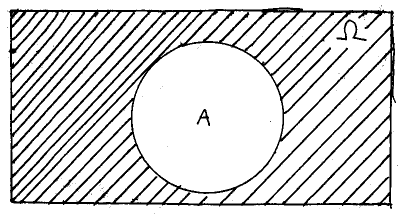
Lastly, the complement of a set A is the set whose elements are contained in the universal set W but not the set A, as below.
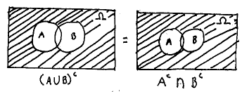
Having been introduced to the basic set operations, you should note that we can combine these operations and extend them to encompass a number of different sets (rather than just two). Therefore, we can define the intersection and complement of an arbitrarily large number of sets (even an infinite number of sets, though we will not discuss this case), and we can also combine these operations in a variety of ways. Some possibilities are illustrated below using Venn diagrams.
Finally, before moving on to probability theory proper, you should also note that we can use the above listed operations to provide a rigorous definition of a subset, which you already know is just a set whose every element is also an element of another set. In terms of our new set theory notation,
Where the iff is to be read "if and only if", the backwards "E" should be read "there exists" and the arrow should be read "implies that".
So what does all this set theory have to do with calculating probabilities anyway? The idea is that we can (tentatively) replace the aforementioned interpretation of probability, which requires actually doing an experiment a large number of times and counting up the number of times some outcome occurs, with a more sophisticated (and less labor-intensive) method. In this method, we count all of the outcomes that could occur in the experiment (if there are a finite number of outcomes) and then count all of the outcomes that are included in the event whose probability we are interested in calculating. Then, we can just divide the number of outcomes included in our "favorable event" set by the total number of outcomes possible. In other words,
where {A} represents the number of sample points in the event set and {W }represents the number of points in the universal set.
Before we apply this however, a few more words about
jargon are in order. It turns out that, due to historical accident, probability
theory has a somewhat different terminology than does set theory. For example,
in probability theory the universal set is called the sample space,
and its elements are called sample points. Therefore, the sample
points represent all of the possible outcomes of an experiment. Additionally,
you should make special note of the fact that only one of these outcomes
can occur per trial. Therefore the sample points represent mutually exclusive
outcomes. Using the notation of set theory, mutually exclusive sets are
those sets which share no elements, i.e. A and B are mutually exclusive
iff ![]() . Such sets are called
disjoint (their intersection is the null set). For example,
in an experiment where we flip a coin once, the possible outcomes are heads
and tails (only one of which may occur per flip). Therefore, the sample
space is given by the set in which each element is a mutually exclusive
outcome and every outcome of the experiment is represented by a sample
point. Occasionally, you will find this last condition referred to as the
exhaustive property of the sample space.
. Such sets are called
disjoint (their intersection is the null set). For example,
in an experiment where we flip a coin once, the possible outcomes are heads
and tails (only one of which may occur per flip). Therefore, the sample
space is given by the set in which each element is a mutually exclusive
outcome and every outcome of the experiment is represented by a sample
point. Occasionally, you will find this last condition referred to as the
exhaustive property of the sample space.
Now, back to our problem of calculating probabilities. As a slight increase in complexity from the last example, lets imagine an experiment where we flip two coins once. Then, the set of all possible outcomes (the sample space) is
To illustrate the utility of the set theoretic approach to computing the probabilities of events (when the state space is finite), consider the probability of the event that you get at least one head in these two flips. Therefore, the probability of this event is

where the notation is the same as in (3).
The subset representing the event we are interested in is
Notice that there are three points in the event set, and four in the sample space. Therefore, assuming all sample points are equiprobable , the probability of getting at least one head in two flips is 3/4=0.75.
While this method of computing probabilities is very useful, it has two major limitations. Namely, it is limited to experiments with a finite sample space and whose sample points are all equiprobable. Unfortunately, it is frequently the case that we are interested in calculating probabilities of events that can not be represented in sample spaces satisfying both of these criteria. However, we can extend the definition of probability much further by defining probability as a function which is defined on all subsets of the sample space that obey certain rules. Although the details of this definition of probability are quite involved, we can boil much of it down to a final definition of probability , as follows:

These axioms are essential to the further discussion of probability and you should therefore be very familiar with them. Briefly, Axiom I. says that probabilities are non-negative. This is rather intuitive, since an event may happen (positive probability), or never happen (zero probability), but can not happen "less than never". Therefore, probabilities are necessarily non-negative for the same reasons that distances, areas and volumes are non-negative (you can never have less than no acres of land or less than no liters of water, etc.). This is not coincidental-probabilities are measures in the mathematical sense, just the same as distances, areas or volumes. Moving on, Axiom II. states that the probability of the state space is unity. All this means is that something must happen in your experiment, and therefore some point in the sample space (which contains all possible outcomes) must be realized. Lastly, and perhaps most importantly for the calculation of probabilities, Axiom III. says that the probability of a union of disjoint (mutually exclusive) events is equal to the sum of the probabilities of the events. This property is sometimes called "countable additivity", and is the starting point of all calculations of probabilities using set theory.
In closing these brief introductory notes on probability theory, we consider the notions of independence of events and conditional probabilities, which are essential to our further discussion of statistics. Intuitively, independent events are those events where the occurrence of one event does not alter the probability of subsequent occurrence of the other. For a more rigorous definition, we define independence as requiring that
 for independent events
 where the capital pi is mathematical shorthand for the product. You have probably already been familiarized with this concept and computation rule, but it wont hurt you to see it again. You should also verify that, in the event of equiprobable outcomes and a finite state space, the result of multiplying probabilities of independent events is identical to that obtained by the "ratio of sample points" method discussed earlier.
Having addressed independent events, we will now turn our attention to computing the probabilities of events which are not independent. For example, given that I roll two dice and the sum of the two faces is 7, what is the probability that I rolled a 6 and a 1 (in that order)? If I did not know the sum of the two faces, then the probability is just (1/6)x(1/6)=1/36 (for two fair dice), by independence. But I do know the sum, and therefore the outcomes of the two die are not independent. This is true because the sum must equal 7, which constrains the admissible outcomes of the experiment. However, we can calculate this probability using a familiar method if we look at the problem somewhat differently. Since not all of the original sample space is relevant to this case (only those outcomes which sum to 7 are), we could construct a new sample space, which is just a subset of the old sample space. This subset would consist of all outcomes of the two dice which sum to 7 (there are six of them, which you should verify), and then every sample point in our new space would be relevant. Then, with this subset as our new sample space, we see that the outcome 6,1 represents 1 of the 6 possible outcomes, and therefore the probability of getting this outcome given the foreknowledge of a sum equal to 7 is 1/6.
In more general terms, the probability of one event
occurring, conditional on the outcome of some other event, is called a
conditional probability. By way of notation, the probability of
A given B is represented ![]() .
Furthermore, we can visualize what a conditional probability represents
by using set theoretic ideas to generalize the method we used above. The
set representing the known outcome (B) represents the sample space. The
event that A occurs given that B occurs is equivalent to the intersection
of sets A and B, i.e.
.
Furthermore, we can visualize what a conditional probability represents
by using set theoretic ideas to generalize the method we used above. The
set representing the known outcome (B) represents the sample space. The
event that A occurs given that B occurs is equivalent to the intersection
of sets A and B, i.e. ![]() .
Therefore, for a finite sample space with equiprobable outcomes,
.
Therefore, for a finite sample space with equiprobable outcomes, ![]() =(the
number of elements in
=(the
number of elements in![]() /the number
of elements in B).
/the number
of elements in B).
However, this method, as used above to calculate a conditional probability suffers from the same limitations that we encountered before with probabilities defined on finite sample spaces and with equiprobable outcomes. We can circumvent these problems in a way exactly analogous to our previous solution; we will work with the probabilities of the subsets explicitly, rather than limiting ourselves to just considering the ratio of numbers of sample points in these sets. Therefore,

Though we will end our discussion of conditional probabilities here, they occupy a central position in the machinery of probability theory and being able to manipulate them is essential to further study in the field.
After this somewhat rushed introduction to probability,
you are now equipped to consider what may be the most important thought-experiment
in the history of probability theory. Statements that grandiose always
sound a bit intimidating, but fear not-one of the most charming aspects
of this experiment is its simplicity. All that it involves is considering
the probability that we get k heads in n flips of a coin. However, for
generality, we will consider a coin that may be loaded (i.e. unfair). By
now you should immediately recognize this means that we can not use our
"ratio of sample points" method because all outcomes in the state space
are no longer equiprobable. However, outcomes of coin-flipping experiments
are an excellent examples of independent trials, and therefore we can just
multiply probabilities. Before progressing, lets take some time to formulate
this problem in a bit more mathematically precise way. The experiment has
two outcomes per flip, with the probability of heads=p and the probability
of tails=q=(1-p). Furthermore, we will be flipping our coin n times, so
each sample point is a list of the n outcomes of these flips. Therefore,
there are 2n sample points in the sample space (not all of which are equiprobable
if p![]() q). Since the outcomes of
each flip are independent, we can just multiply the probabilities for these
two outcomes, and get
q). Since the outcomes of
each flip are independent, we can just multiply the probabilities for these
two outcomes, and get
The bad news is that this probability is dramatically less than the true probability. What have we done wrong? Recall that the sample points are lists of the outcomes of the n flips. Since order matters in a list, the results (hhhtth) and (hhthth) would represent two distinct outcomes (and therefore sample points), even though they have the same number of heads and tails. Therefore, the reason our calculation of the probability above is wrong is that we have not taken into account the fact that there are many different sample points included in the subset corresponding to obtaining k heads in n flips. Therefore, we need to multiply the probability above by the number of ways there are to get k heads in n flips (which is equivalent to the number of sample points in our event set).
Now we must confront a difficulty. We could count these outcomes by writing out every sample point (sequence of outcomes) for the flips, and then count those that have k heads, but this gets practically impossible for even a modest number of flips (remember the number of points in the sample space is 2n). However, we can proceed by making use of some results from a field of mathematics called combinatorics. Looking at the problem somewhat differently, we are asking "how many different arrangements (mathematicians call them permutations) of k objects of one kind (heads) and n-k objects of another kind (tails) can we achieve"? The important point here is that we must consider each of the n flips as distinct, rather than just recording whether we got a head or a tail. To make this explicit, you might imagine that we have numbered every flip in addition to recording the outcome. This means that we have n choices for the first position, since any one of the n results can be placed in that position. However, for the next choice, we have only (n-1) possibilities, and for the subsequent choice (n-2), etc., since every choice depletes our "pool" of subsequent choices by one. Therefore there are n!=(n)(n-1)(n-2)...(1) permutations of n distinguishable objects. However, consider the two permutations (h1t2t3h4h5) and (h4t3t2h1h5), where the subscript numbers indicate the numbered outcomes discussed above. From a permutation standpoint these are distinct outcomes, but for our purposes they are identical, since they both represent the sequence (htthh). Therefore, we have overcounted the number of distinct sequences because we have considered every outcome (every head and every tail) as distinguishable. Since we are only concerned with how many sequences of k heads and n-k tails there are, without regard to which head or which tail we are talking about, we need to divide n! by the number of ways that we can switch around all of the numbered heads and tails and still preserve the sequence. We now know that for k heads, there are k! permutations, and likewise (n-k)! permutations for the tails. Therefore, there are

different sequences of k heads and (n-k) tails. In combinatorial parlance, these distinct sequences with which we are concerned are called combinations, to distinguish them from the aforementioned permutations. This means that the true probability is

The expression above is a venerated distribution in discrete probability. It is called the binomial distribution, and it crops up so frequently in such diverse applications that we need no further justification for emphasizing it. However, in addition to being important in its own regard, the binomial distribution also marks a critical juncture in the development of probability theory. To see why, consider the presence of the factorial terms in the binomial coefficient. They are problematic since these terms grow rapidly as n increases, making calculation of the binomial coefficient challenging (especially in a pre-computer era) for n greater than 10 or so. Therefore, rather than explicitly evaluating this expression if n is large, we would like to find some function which closely approximates the binomial distribution when n is large. In addition to closely approximating the binomial distribution, this function may be continuous (for convenience) and should be valid within a wide range of values for p (the probability of "success" in our Bernoulli trial). Unfortunately, there is no single function which satisfies the last two of these criteria, but we can find a set of two functions (one continuous and one discrete) that satisfy all of these criteria. These functions are the normal (Gaussian) and Poisson distributions (respectively), and we will shortly turn our attention to both.
However, before moving on to discuss these distributions, we should take some time to briefly discuss a new idea that was introduced with the binomial distribution. Recall that we were concerned with calculating the probability of getting k heads in n flips of a coin. Though there was a subset of sample points which satisfied this criterion, we needed to recognize how the variable "get k heads in n trials" depended on these sample points. Similarly, we might have discussed the probability that I make $5 if I make $0.50 on each head and the coin is tossed n times. While this quantity depends on the outcomes of the flips (sample points), it is not one of them. Therefore, we have introduced the idea of a quantity which may be regarded as a function of the sample points, where the sample points act as the independent variable. Such a quantity is called a random variable, and it is essential that you be familiar with this concept before we move on to discussing various probability distributions. To gain some practice with the concept, imagine some other random variables that we could use in conjunction with the binomial distribution. Hopefully, you will appreciate that there are an infinite number of them, and therefore you should expect that most applications of probability theory to real life involve dealing directly with random variables rather than sample points.
Having introduced the idea of approximating the binomial
distribution with two distributions, each of which is applicable in a different
regime of the value of p, lets consider the case where p is small (p![]() 0.1).
First, let us perform the substitution l
=np. The binomial distribution then becomes,
0.1).
First, let us perform the substitution l
=np. The binomial distribution then becomes,

Now, consider the case where n grows to infinity and p shrinks to zero. Hopefully you appreciate the utility of the substitution that we made above, since we can force n to grow and p to shrink such that l =np remains constant. This is nice since nothing in the above expression will "blow up" for large n and/or small p. In this limit we get,
 for k=0,1,2,3,...
This expression is the Poisson distribution, and is useful in the situations where the probability of an occurrence is small and the number of "trials" (n) is large. For example, we might consider the probability of k adverse reactions to a test drug in a given sample of the population or the probability of registering k complaints about a particular product in a 1-hour period or the probability of finding k point mutations in a given stretch of nucleotides. Though the Poisson distribution is essential to application and you will doubtless see it again, we will leave it now to discuss the other binomial-approximating continuous distribution.
If the probability of success in a Bernoulli trial is not sufficiently small to justify the assumptions that went into the derivation of the Poisson distribution, then we may derive an alternative approximating distribution. It can be shown that this distribution is continuous and given by
 for
for This is the normal (or Gaussian) distribution. You are already familiar with this distribution from course grading (as well as much else), and it looms over probability theory as the single most important continuous distribution in applications. It is so significant that it can be proven that every distribution approaches a normal distribution under suitable limits.
As where the Poisson distribution was characterized
by a single parameter, l
, the normal distribution is characterized by two quantities; the mean
m and the variance ![]() .
The mean is just a generalization of the notion of an average, whereby
we weight every value that the random variable (r.v.) can attain by the
probability that this particular value is realized. In other words,
.
The mean is just a generalization of the notion of an average, whereby
we weight every value that the random variable (r.v.) can attain by the
probability that this particular value is realized. In other words,

where ![]() are all of the values that the r.v. can attain and
are all of the values that the r.v. can attain and ![]() is the probability that the r.v. achieves a value
is the probability that the r.v. achieves a value ![]() .
In addition, you should verify that in the case that all values of the
are equiprobable, the mean reduces to the arithmetic average. Therefore,
the mean is just a weighted average. Furthermore, the mean is often called
a "measure of location", which makes sense given that the normal distribution
is centered around the mean. However, for non-symmetric distributions,
there are two other measures of location that become non-redundant with
the mean. These alternative measures of location are the median and the
mode. The median is the value of the r. v. where there are equal numbers
of observations with values greater and less than the median. The mode
is the most frequently observed single value of the r. v. These are of
little relevance to the normal distribution, but are often of significant
value when dealing with data for statistical purposes.
.
In addition, you should verify that in the case that all values of the
are equiprobable, the mean reduces to the arithmetic average. Therefore,
the mean is just a weighted average. Furthermore, the mean is often called
a "measure of location", which makes sense given that the normal distribution
is centered around the mean. However, for non-symmetric distributions,
there are two other measures of location that become non-redundant with
the mean. These alternative measures of location are the median and the
mode. The median is the value of the r. v. where there are equal numbers
of observations with values greater and less than the median. The mode
is the most frequently observed single value of the r. v. These are of
little relevance to the normal distribution, but are often of significant
value when dealing with data for statistical purposes.
Whereas the mean provides information concerning the location of the distribution, the variance provides information concerning the "spread" of the distribution about the mean. In particular,

You may be more familiar with the standard deviation, which is related to the variance as below.
Thus, the standard deviation (std. dev.) is just the average difference between the mean and the observed values of the r.v. Therefore, if we are considering a set of observations that we believe are normally distributed, then the std. dev. (or the variance) provide a measure of the variability of observations.
Having introduced the normal distribution, we have yet to deal with a problem created by our shift from the discrete binomial distribution to the continuous normal distribution. Specifically, while we can speak of the probability that a r.v. equals a particular value with a discrete distribution over a finite sample space, we can not do so when dealing with a continuous distribution. This is because a continuous distribution has an infinite number of sample points, and therefore the probability that one value is realized is always zero (because you have one point in your event set and an infinite number in your sample space). Therefore, when dealing with continuous distributions, we can only speak of the probability that the r.v. takes on a value in a certain range. Therefore, taking the normal distribution as an example,

We see that to determine the probability that the r. v. falls within a range we must integrate these distributions. The functions F(a) and F(b) are called cumulative distribution functions, and are just integrated probability distributions. The function f(X), which we have thus far called a probability distribution, is more properly called a probability density. This name is suggestive of an analogous shift from a discrete to a continuous treatment of mass in physics. For a small number of particles, we can treat matter as comprised of discrete mass points. For larger numbers of particles, we abandon this approach in favor of describing matter using a continuous function called a mass density. Similarly, we describe continuous probability distributions using probability density functions. To extend the aforementioned definitions of mean and variance to the continuous case,
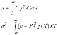
These expressions look very similar to expressions for the center of mass and moment of inertia for continuous mass distributions from physics. You now know that this not coincidental.